In the last post we took our first step in the mathematical introduction to classical Mechanics. In this post we’ll introduce a few physical concepts and some more mathematical tools.
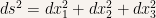
— 1. Velocity and Acceleration —
The first thing to notice is that in Physics velocity is a vector concept. That means that in order for us to specify the velocity of an entity we must not only indicate its magnitude but also its direction.
First of we need to define a frame.
| Definition 1
A frame is a set of axis and a special point that is taken as the origin that allows one to describe the motion of a particle. |
When to get to real Physics we’ll talk a little bit more of what is a particle in Physics but for now we’ll just leave it to intuition and/or background knowledge.
If we trace the position of a particle for a given period of time what we get is curve whose parameter is time and this curve has the name of trajectory.
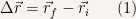
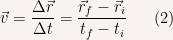
If we want to keep track of the variations of the position of a particle when it is describing a given trajectory we can do that using the concept of displacement.
Definition 2 Displacement is the difference between the final and initial positions of a particle. It is represented by the symbol  and is calculated in the following way: and is calculated in the following way:
|
Now we all know that when a body describes a trajectory some parts of it may take a longer time and others a shorter time. To rigorously describe the notion of a particle we have to take into account its variability in the motion and we do this by introducing the concept of velocity.
| Definition 3
The average velocity of a particle is the rate of change in position of a particle for a given time interval.
|
| Definition 4
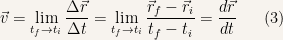
Sometimes we aren’t interested in the average velocity and we want to know what is the velocity of a particle in a given instant. Intuitively we know that if we measure the average velocity in a sufficiently small interval we won’t be making a very big error in determining the value of the velocity.
If we let the time interval go to to zero what the have is the velocity of the particle for the instant considered. We can be rest assured that such a limit always exist since we are dealing with real bodies and their movements are always smooth.
|
Another way to mathematically define the average velocity and velocity is to make a change of variable and define  and calculate
  ,
,  and
and  .
.
The other quantity of physical interest is average acceleration and it is the the rate of change in velocity of a particle in a given time interval.
The definitions are analogous to the ones of average velocity and we just have to change  to
to  .
.
We’ll just state the equation for acceleration here:
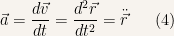
Where  is the so called Newton notation and indicates that we are differentiating two times with respect to
  . Obviously that one dot indicates that we are differentiating one time, and etc.
If we use Cartesian coordinates we know that it is  . Since our basis vectors are fixed it follows that
 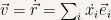 and that
  .
.
— 2. Curvilinear Coordinates —
Sometimes to use Cartesian Coordinates in order to describe the motion of a particle is very awkward and one instead uses some other kind of curvilinear coordinates. The ones that are most used are, polar coordinates, cylindrical coordinates and spherical coordinates.
— 2.1. Polar Coordinates —
If we are dealing with two dimensional problems that have circular symmetry then the best way to deal with them is to use polar coordinates.
In this system of coordinates instead of the  and
and  coordinates, one uses a radial coordinate
  that expresses the distance that a point is from the origin and an angular coordinate
  . This angular coordinate is measured from the
  axis to the position vector in counter clockwise direction.
The range of values for these two variables are  and
and  . Notice that in
  isn’t defined and thus the origin can be thought to be a kind of singularity, but this is only so because we chose a particular set of coordinate and it isn’t intrinsic to the point itself.

As indicated in the picture the transformation of coordinates is:
— 2.2. Cylindrical Coordinates —
Sometimes when dealing with three dimensional problems we have to deal with circular symmetry around a certain axis. If this happens the most apt way to deal with the said problem is to use cylindrical coordinates.
Again we’ll use a mix of radial distances and angular distances. First we’ll only think about the plane formed by the and axes. In this plane we’ll project the position vector of a given point. The angle between and this projection is . The other two coordinates are which is the distance between the point in question and the origin, and  (or
(or  ).
).

The range of values for these three coordinates are  , and
, and  ,
,
As indicated in the pictures the transformation of coordinates is:
— 2.3. Spherical Coordinates —
The last kind of curvilinear coordinates that we’ll look at are spherical coordinates. This kind of coordinates are extremely useful when a problem has spherical symmetry.
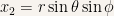
This time we’ll have one radial coordinate and two angular coordinate. Like we did for cylindrical coordinates first we’ll project the position vector into the , plane and define  to be the angle between and the projection of the position vector. is the distance between the origin and the point in question. The second angular coordinate is and it is measured between and the position vector.

As can be seen from the picture the change of variables from spherical coordinates to Cartesian coordinates is:
The range of each coordinate is defined to be ,  and
and  .
.
— 3. Velocity and Acceleration in Curvilinear Coordinates —
Having defined the previous three systems of coordinates it is time for us to know how to write the velocity and acceleration of a particle in these systems of coordinates.
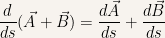
As we already saw for Cartesian coordinates one has the following relationships:
Our task will be to see how these equations translate when we are dealing with polar, cylindrical and spherical coordinates.
— 3.1. Polar Coordinates —
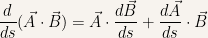
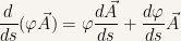
Has stated previously when we are using curvilinear coordinates the basis vector change from point to point. Hence one has to use Leibniz rule when calculating derivatives.
If we have two points that are infinitely close to each other,  and
and  (the reason for using superscripts will be evident right away) the infinitesimal variation in
  is
is  and for the angular infinitesimal variation it is
The previous relationships allows one to see that the infinitesimal variation for is perpendicular to and that the infinitesimal variation for  is perpendicular to . One can show this rigorously but I’ll only state the result that it is
Hence

Thus the velocity can be thought has having a radial component and an angular component. The radial component is  and is a measure for the variation of velocity in magnitude. The radial component is
  and it measures the rate of change in direction for the position vector.
The  term is so important and appears so many times that it deserves its own special name. It called the angular velocity, it is represented by the symbol
  and if one is interested in an vector representation it is
  .
.
For the acceleration it is

Hence the radial component of the acceleration is  and the angular component is
  .
.
— 3.2. Cylindrical Coordinates —
For cylindrical coordinates the infinitesimal line element is  . Hence one can show that it is
— 3.3. Spherical Coordinates —
For spherical coordinates the infinitesimal line element is  . And for the velocity it is
— 4. Vector Calculus —
In this part of our post we’ll take a very brief look at some concepts of vector calculus that are useful to Physics.
— 4.1. Gradient, Divergence and Curl —
If one has  a scalar function, continuous and differentiable, it is by definition
  . From this it follows
The inverse coordinate transformation is  . If we calculate the derivative of
  with respect to
  it is
it is

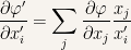
Hence it is  . From what we’ve seen in the last post this means that the function
  is the j-th component of a vector.
If we introduce the operator  (sometimes called del) whose definition is

we can define the gradient of a scalar function,  to be
to be 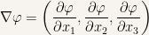 .
.
The divergence of a vector field,  , is a scalar and is defined to be:

If the divergence of vector field is positive at a given point that means that in that point a source of the field is present. If the divergence of the field is negative that means that a sink of the field is present.
Another vector entity that one can define with the del operator is the curl of a vector field. The curl is a vector entity too and its definition is:

The last operator that we’ll define in this section is the Laplacian. This operator is the result of applying the del operator two times and it is


 that is rotated relatively to
  that has coordinates
  on
on  on
on  ,
,  and that
  .
.

 case.
case.
 to
to  and we get the first equation. For the other two a similar reasoning applies.
 indexes can be arranged in a form of a matrix:


 is a matrix known as Kronecker delta and its definition is
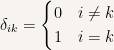
 it is
it is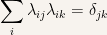


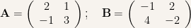
 , to be possible only when the number of columns of
  is equal to the number of rows of
 , we will denote this element by the symbol
  is,
is,![\displaystyle \mathbf{C}_{ij}=[\mathbf{AB}]_{ij}=\sum_k A_{ik}B_{kj}](https://s0.wp.com/latex.php?latex=%5Cdisplaystyle++%5Cmathbf%7BC%7D_%7Bij%7D%3D%5B%5Cmathbf%7BAB%7D%5D_%7Bij%7D%3D%5Csum_k+A_%7Bik%7DB_%7Bkj%7D+&bg=f7f3ee&fg=000000&s=0&c=20201002)


 is the transposed of
  . In a more pedestrian way one can say that in order to obtain the transpose of a given matrix one needs only to exchange its rows and columns.
 such as
  . The matrix
  .
. , then
  ,
,  .
.
 .
. . Also matrix addition has just the definition one would expect. Namely
  .
.
 and that the inversion matrix has a
  determinant we know that there isn’t any continuous transformation that maps a rotation into an inversion.
 , if it is:
 then
then  for
for  ,
,  and
and  then
then  is said to be a vector.


 is a vector.
 is a scalar.
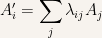
 transforms like a vector.
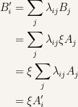
 and
and  , where one changes the index of the second summation because we’ll have to multiply the two quantities and that way the final result can be achieved much more easily.
 is a scalar.
 . Its definition is
  if two or three of its indices are equal;
  if
if  is an even permutation of
  (the even permutations are
  and
and  );
);  if
if  ,
,  and
and  ).
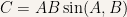
). , of two vectors
  is denoted by
  .
.
 is shorthand notation for
  .
.

 throughout the reasoning.
 and that
  .
. .
. any vector
  . We also have that
  and
and  . Another way to write the last equation is
 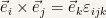 .
. :
:  . Since both
  and
and  . Hence it also is
  and
and 
 .
. hence
hence

 transforms like the coordinates of a vector which is the same as saying that
  is a vector.