


Exercise 2 Consider the first  digits in the decimal expansion of digits in the decimal expansion of  . .
|


 . The median digit is
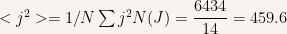
  . The average is
  .
.

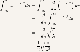
Exercise 3 The needle on a broken car is free to swing, and bounces perfectly off the pins on either end, so that if you give it a flick it is equally likely to come to rest at any angle between  and . and .
|
![{\left[0,\pi\right]}](https://s0.wp.com/latex.php?latex=%7B%5Cleft%5B0%2C%5Cpi%5Cright%5D%7D&bg=f7f3ee&fg=000000&s=0&c=20201002) interval the probability of the needle flicking an angle
interval the probability of the needle flicking an angle  is
is  . Given the definition of probability density it is
  .
.


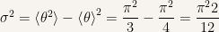
 ,
,  and
and  .
.
![{\begin{aligned} \left\langle\theta \right\rangle &= \int_0^\pi\frac{\theta}{\pi}d\theta\\ &= \frac{1}{\pi}\int_0^\pi\theta d\theta\\ &= \frac{1}{\pi} \left[ \frac{\theta^2}{2} \right]_0^\pi\\ &= \frac{\pi}{2} \end{aligned}}](https://s0.wp.com/latex.php?latex=%7B%5Cbegin%7Baligned%7D+%5Cleft%5Clangle%5Ctheta+%5Cright%5Crangle+%26%3D+%5Cint_0%5E%5Cpi%5Cfrac%7B%5Ctheta%7D%7B%5Cpi%7Dd%5Ctheta%5C%5C+%26%3D+%5Cfrac%7B1%7D%7B%5Cpi%7D%5Cint_0%5E%5Cpi%5Ctheta+d%5Ctheta%5C%5C+%26%3D+%5Cfrac%7B1%7D%7B%5Cpi%7D+%5Cleft%5B+%5Cfrac%7B%5Ctheta%5E2%7D%7B2%7D+%5Cright%5D_0%5E%5Cpi%5C%5C+%26%3D+%5Cfrac%7B%5Cpi%7D%7B2%7D+%5Cend%7Baligned%7D%7D&bg=f7f3ee&fg=000000&s=0&c=20201002)
![{\begin{aligned} \left\langle\theta^2 \right\rangle &= \int_0^\pi\frac{\theta^2}{\pi}d\theta\\ &= \frac{1}{\pi} \left[ \frac{\theta^3}{3} \right]_0^\pi\\ &= \frac{\pi^2}{3} \end{aligned}}](https://s0.wp.com/latex.php?latex=%7B%5Cbegin%7Baligned%7D+%5Cleft%5Clangle%5Ctheta%5E2+%5Cright%5Crangle+%26%3D+%5Cint_0%5E%5Cpi%5Cfrac%7B%5Ctheta%5E2%7D%7B%5Cpi%7Dd%5Ctheta%5C%5C+%26%3D+%5Cfrac%7B1%7D%7B%5Cpi%7D+%5Cleft%5B+%5Cfrac%7B%5Ctheta%5E3%7D%7B3%7D+%5Cright%5D_0%5E%5Cpi%5C%5C+%26%3D+%5Cfrac%7B%5Cpi%5E2%7D%7B3%7D+%5Cend%7Baligned%7D%7D&bg=f7f3ee&fg=000000&s=0&c=20201002)
 .
. .
. ,
,  and
and  .
.
![{\begin{aligned} \left\langle\sin\theta \right\rangle &= \int_0^\pi\frac{\sin\theta}{\pi}d\theta\\ &= \frac{1}{\pi}\int_0^\pi\sin\theta d\theta\\ &= \frac{1}{\pi} \left[ -\cos\theta \right]_0^\pi\\ &= \frac{2}{\pi} \end{aligned}}](https://s0.wp.com/latex.php?latex=%7B%5Cbegin%7Baligned%7D+%5Cleft%5Clangle%5Csin%5Ctheta+%5Cright%5Crangle+%26%3D+%5Cint_0%5E%5Cpi%5Cfrac%7B%5Csin%5Ctheta%7D%7B%5Cpi%7Dd%5Ctheta%5C%5C+%26%3D+%5Cfrac%7B1%7D%7B%5Cpi%7D%5Cint_0%5E%5Cpi%5Csin%5Ctheta+d%5Ctheta%5C%5C+%26%3D+%5Cfrac%7B1%7D%7B%5Cpi%7D+%5Cleft%5B+-%5Ccos%5Ctheta+%5Cright%5D_0%5E%5Cpi%5C%5C+%26%3D+%5Cfrac%7B2%7D%7B%5Cpi%7D+%5Cend%7Baligned%7D%7D&bg=f7f3ee&fg=000000&s=0&c=20201002)
![{\begin{aligned} \left\langle\cos\theta \right\rangle &= \int_0^\pi\frac{\cos\theta}{\pi}d\theta\\ &= \frac{1}{\pi}\int_0^\pi\cos\theta d\theta\\ &= \frac{1}{\pi} \left[ \sin\theta \right]_0^\pi\\ &= 0 \end{aligned}}](https://s0.wp.com/latex.php?latex=%7B%5Cbegin%7Baligned%7D+%5Cleft%5Clangle%5Ccos%5Ctheta+%5Cright%5Crangle+%26%3D+%5Cint_0%5E%5Cpi%5Cfrac%7B%5Ccos%5Ctheta%7D%7B%5Cpi%7Dd%5Ctheta%5C%5C+%26%3D+%5Cfrac%7B1%7D%7B%5Cpi%7D%5Cint_0%5E%5Cpi%5Ccos%5Ctheta+d%5Ctheta%5C%5C+%26%3D+%5Cfrac%7B1%7D%7B%5Cpi%7D+%5Cleft%5B+%5Csin%5Ctheta+%5Cright%5D_0%5E%5Cpi%5C%5C+%26%3D+0+%5Cend%7Baligned%7D%7D&bg=f7f3ee&fg=000000&s=0&c=20201002)
 as an exercise for the reader. As a hint remember that
  .
.
Exercise 4
|
 it was shown that the the probability density is

 is
is
 it is
it is![{\begin{aligned} \left\langle x^2 \right\rangle &= \int_0^h\frac{x}{2\sqrt{hx}}dx\\ &= \frac{1}{2\sqrt{h}}\int_0^h x^{3/2}dx\\ &= \frac{1}{2\sqrt{h}}\left[\frac{2}{5}x^{5/2} \right]_0^h\\ &= \frac{h^2}{5} \end{aligned}}](https://s0.wp.com/latex.php?latex=%7B%5Cbegin%7Baligned%7D+%5Cleft%5Clangle+x%5E2+%5Cright%5Crangle+%26%3D+%5Cint_0%5Eh%5Cfrac%7Bx%7D%7B2%5Csqrt%7Bhx%7D%7Ddx%5C%5C+%26%3D+%5Cfrac%7B1%7D%7B2%5Csqrt%7Bh%7D%7D%5Cint_0%5Eh+x%5E%7B3%2F2%7Ddx%5C%5C+%26%3D+%5Cfrac%7B1%7D%7B2%5Csqrt%7Bh%7D%7D%5Cleft%5B%5Cfrac%7B2%7D%7B5%7Dx%5E%7B5%2F2%7D+%5Cright%5D_0%5Eh%5C%5C+%26%3D+%5Cfrac%7Bh%5E2%7D%7B5%7D+%5Cend%7Baligned%7D%7D&bg=f7f3ee&fg=000000&s=0&c=20201002)


![{\left[0,\left\langle x \right\rangle+\sigma\right]}](https://s0.wp.com/latex.php?latex=%7B%5Cleft%5B0%2C%5Cleft%5Clangle+x+%5Cright%5Crangle%2B%5Csigma%5Cright%5D%7D&bg=f7f3ee&fg=000000&s=0&c=20201002) and the second is
and the second is ![{\left[\left\langle x \right\rangle+\sigma,h\right]}](https://s0.wp.com/latex.php?latex=%7B%5Cleft%5B%5Cleft%5Clangle+x+%5Cright%5Crangle%2B%5Csigma%2Ch%5Cright%5D%7D&bg=f7f3ee&fg=000000&s=0&c=20201002) .
.
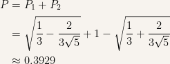
 denote the probability of the first interval and
  denote the probability of the second interval.
![{\begin{aligned} P_1 &= \int_0^{\left\langle x \right\rangle-\sigma}\frac{1}{2\sqrt{hx}}dx\\ &= \frac{1}{2\sqrt{h}}\left[2x^{1/2} \right]_0^{\left\langle x \right\rangle-\sigma}\\ &= \frac{1}{\sqrt{h}}\sqrt{\frac{h}{3}-\frac{2h}{3\sqrt{5}}}\\ &=\sqrt{\frac{1}{3}-\frac{2}{3\sqrt{5}}} \end{aligned}}](https://s0.wp.com/latex.php?latex=%7B%5Cbegin%7Baligned%7D+P_1+%26%3D+%5Cint_0%5E%7B%5Cleft%5Clangle+x+%5Cright%5Crangle-%5Csigma%7D%5Cfrac%7B1%7D%7B2%5Csqrt%7Bhx%7D%7Ddx%5C%5C+%26%3D+%5Cfrac%7B1%7D%7B2%5Csqrt%7Bh%7D%7D%5Cleft%5B2x%5E%7B1%2F2%7D+%5Cright%5D_0%5E%7B%5Cleft%5Clangle+x+%5Cright%5Crangle-%5Csigma%7D%5C%5C+%26%3D+%5Cfrac%7B1%7D%7B%5Csqrt%7Bh%7D%7D%5Csqrt%7B%5Cfrac%7Bh%7D%7B3%7D-%5Cfrac%7B2h%7D%7B3%5Csqrt%7B5%7D%7D%7D%5C%5C+%26%3D%5Csqrt%7B%5Cfrac%7B1%7D%7B3%7D-%5Cfrac%7B2%7D%7B3%5Csqrt%7B5%7D%7D%7D+%5Cend%7Baligned%7D%7D&bg=f7f3ee&fg=000000&s=0&c=20201002)

 is
is 
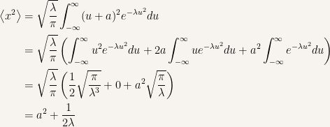
Exercise 5 The probability density is 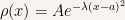
|
 .
.
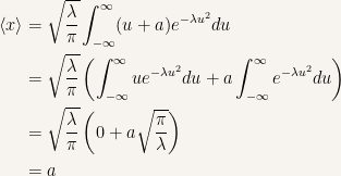
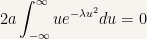
 (
( ) the normalization condition is

 ,
, 
 check
check 
 as in the previous calculation.
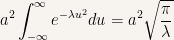 .
.


— Mathematica file —
The resolution of exercise 2 was done using some basic Mathematica code which I’ll post here hoping that it can be helpful to the readers of this blog.
// N[Pi, 25]piexpansion = IntegerDigits[3141592653589793238462643]
digitcount = {}
For[i = 0, i <= 9, i++, AppendTo[digitcount, Count[A, i]]]
digitcount
digitprobability = {}
For[i = 0, i <= 9, i++, AppendTo[digitprobability, Count[A, i]/25]]
digitprobability
digits = {}
For[i = 0, i <= 9, i++, AppendTo[digits, i]]
digits
j = N[digits.digitprobability]
digitssquared = {}
For[i = 0, i <= 9, i++, AppendTo[digitssquared, i^2]]
digitssquared
jsquared = N[digitssquared.digitprobability]
sigmasquared = jsquared - j^2
std = Sqrt[sigmasquared]
deviations = {}
deviations = piexpansion - j
deviationssquared = (piexpansion - j)^2
variance = Mean[deviationssquared]
standarddeviation = Sqrt[variance]
