— 1. Variational Calculus —
| Definition 1 A functional is a mapping from vector spaces to into real numbers. |
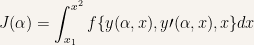
Let 


According to definition 1 

Let 


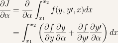
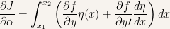
We can write 


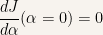
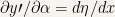
Now
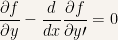
Therefore the condition for
 . Take
 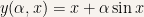 as a parametric representation of
  ,
,  and
and  .
.
 and
and 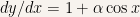 .
. .
. it is trivial to see that the minimum value is reached when
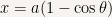
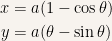
Exercise 1 Given the points 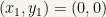 and and  , calculate the equation of the curve that minimizes the distance between the points , calculate the equation of the curve that minimizes the distance between the points
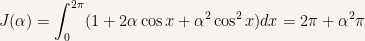
Now It is And it is The rest is left as an exercise for the reader. |
 .
. ,
, 
 with
with  .
.— 2. Euler Equations —
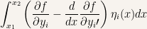
In the following section we’ll analyze the condition for
Since it is 
Now 
For the first term it is 
Hence

Remembering that 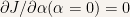
The previous equation is known as the Euler’s Equation
 and goes to point
  .
.
 . Let us take our original point as being our reference point for the potential. Then it is
  .
. . For the potential it is
  . From the previous equations it follows that
  .
.
 since
since  is only a constant factor and can be omitted from our analysis. Given the functional form of
  and Euler’s Equation just is:
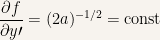

 it follows
  . Hence the expression for
  . Since our particle starts from the origin it is
  .
.
To close our thoughts on the Euler equation let us say that there also is a second form for the Euler equation. The second form is
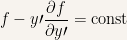
and is used in the cases where
— 3. Euler Equation for 
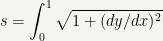
Let 
Now we have 


That is to say we have
— 4. Hamilton’s Principle —
Minimum principles have a long history in the history of Physics:
- Heron explained the law of light reflection using a principle of minimum time.
- Fermat corrected Heron’s Principle by stating that light travels between two points in the shortest time available.
- Maupertuis stated his minimum action principle that postulated that a particle’s dynamics always minimized the action.
- Gauss postulated his principle of least constraint.
- Hertz postulaed his principle of minimum curvature.
In modern Physics one uses a more general extremum principle and the focus of this section will be to state this principle and flesh out its consequences.
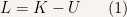
Definition 2 The lagrangian (sometimes called the lagrangian function),  , of a particle is the difference between its kinetic and potential energies. , of a particle is the difference between its kinetic and potential energies.
|
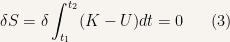
Definition 3 The action,  , of a particle’s movement (be it a real or virtual one) is: , of a particle’s movement (be it a real or virtual one) is:
|

Axiom 1 Given a collection of paths that a particle can take between points and in the the time interval  the actual path that the particle takes is the one that makes the action stationary the actual path that the particle takes is the one that makes the action stationary
|
For rectangular coordinates it is 

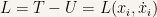

The function


In this case the Euler equations are called the Euler-Lagrange equations and it is
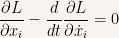
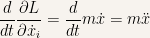
| Example 3 Let us study the harmonic oscillator under Langrangian formalism
First it is Then we have Hence it is |

 .
. .
.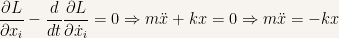 which is just the harmonic oscillator dynamic equation that we already know.
| Example 4 Consider a planar pendulumplanar pendulum write its Lagrangian and derive its equation of motion.
The Lagrangian for the planar pendulum is If we consider This is precisely the equation of motion of a planar pendulum and this result is apparently unexpected since we only analyzed the Lagrangian for rectangular coordinates. |

 to be a rectangular coordinate (which it isn’t!) it follows that the equation of motion is:
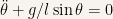
— 5. Generalized coordinates —
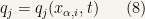
Consider a mechanical system constituted by 


Let 

| Definition 4 The set of coordinates that totally specify the mechanical state of particles is defined to be the set of generalized coordinates.
The generalized coordinates are represented by |

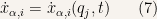
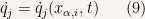
Since we defined the generalized coordinates of a system of particles one can also define its set of generalized velocities.

Let 


For the generalized velocities it is
The inverse transformations are
and
Finally let us note that we also need 
with 
 whose center is the origin of the coordinate system.
 and
and  .
. ,
,  and
and  be our generalized coordinates.
 as a constraint equation. Hence
| Definition 6 Configuration space is the vector space defined by the generalized coordinates |
The time evolution of a mechanical system can be represented as a curve in the configuration space.
— 6. Euler-Lagrange Equations in generalized coordinates —
Since 

Hence it is

and 
Hence we can write Hamilton’s Principle (Section 4) in the form
That is


are the analogies to be made now.
Finally the Euler-Lagrange Equations are

for
To finalize this section let us note the conditions of validity for the Euler-Lagrange equations:
- The system is conservative.
- The equations of constraint have to be functions between the coordinates of the particles and can also be a function of time.

 and
and 
 . Thus the lagrangian is
 it is
it is  . Hence it is
  .
. axis is
  . Thus
  expresses the conservation of angular momentum about the axis of symmetry of system.
 .
.