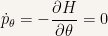
— 7. Newton and Euler-Lagrange Equations —
We’ve seen in the previous examples that solving a problema while using the lagrangian formalism would lead us to the same equations of Newton’s formalism.
In this section we’ll show that both formulations are indeed equivalent for conservative systems.
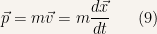
We have 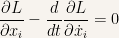 for
for  . The previous equation can be written in the following form:
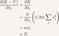
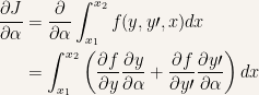
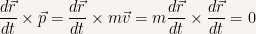
Since our analysis doesn’t depend on the type of coordinates one uses we’ll choose to use rectangular coordinates. Hence it is  and
and  . It is
  and
and  . Hence
  . Since for a conservative system it is
  it follows that
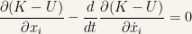
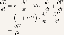
 Finally it is
  which is Newton’s Second Axiom. Since the dynamics of a particle are a result of this axiom the dynamics of a given particle have to be the same on both formulations of mechanics.
— 8. Symmetry considerations —
As you certainly noticed in the previous examples the absence of generalized coordinate on the lagrangian of the system implied the conservation of a momentum (angular or linear). These coordinates that don’t appear on the lagrangian are called cyclic coordinates in the literature.
Obviously that the presence or absence of cyclical coordinates on a lagrangian depend on the choice of coordinate that one makes. But the fact that a moment is conserved cannot depend on the choice of the set of coordinates one makes.
Since the right choice of coordinates is linked to the symmetry that the system exhibits one can conclude that symmetry and conserved quantities are intrinsically connected.
In this section we’ll understand why symmetry considerations are so important in contemporary Physics and what is the relationship between symmetry and conservation. If a system exhibits some kind of continuous symmetry this symmetry will always manifest in the form some conserved quantity. The mathematical proof of this theorem (and its multiple generalizations) is Noether’s theorem and I won’t provide a proof of it here. Instead we’ll look into the consequences of three types of continuous symmetry and I’ll provide you links for you to study Noether’s theorem:
— 8.1. Continuous symmetry for time translations —
As we saw in Newtonian Mechanics 01 a frame is said to be inertial if time is homogeneous. When one says that time is homogeneous one is saying that one can perform a continuous time translation (formally one says  ) and the characteristics of the mechanical system won’t change.
Let  denote the lagrangian of an isolated system. Since the system is isolated its physical characteristics must remain unchanged for all times. This is equivalent to saying that the lagrangian can’t depend on time (
 .)
.)
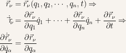
Hence the total derivative is just
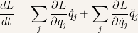
Using Euler-Lagrange equations 13 for generalized coordinates it is

In conclusion it is
where  (the
(the  sign will be apparent later) is some constant.
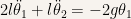
Suppose that  and
and  . Then it is
  and
and  . Hence
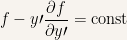
Then we can write equation 14 as  . From this it follows
  .
.
The function  is called the Hamiltonian and its definition is given by equation 14.
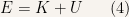
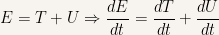
Furthermore one can identify the Hamiltonian with the total energy of the system if the following conditions are met:
- The equations of coordinate transformations are time independent which implies that the kinetic energy is a quadratic homogeneous function of

- The potential energy is velocity independent so that the terms
 can be eliminated.
— 8.2. Continuous symmetry for space translations —
As we saw in Newtonian Mechanics 01 a frame is said to be inertial if space is homogeneous. When one says that space is homogeneous one is saying that the lagrangian is invariant under space translations. Formally one says that  for
for  .
.
Without loss of generality let us consider just one particle. Now  and
and  . In this case the variation in due to
  is
is
Now  so the expression for the variation in the lagrangian becomes
For the previous expression to be identically  one has to have
  since the
  are arbitrary variations.
According to Euler-Lagrange equations 13 one also has  .
.
Hence the homogeneity of space to translations implies the conservation of linear momentum in an isolated system.
— 8.3. Continuous symmetry for space rotations —
As we saw in Newtonian Mechanics 01 a frame is said to be inertial if space is isotropic. When one says that space is isotropic one is saying that the lagrangian is invariant under space rotations. Formally one says that for where  .
.
First we have (we’re considering one particle) 
From  and
and  it follows

Since 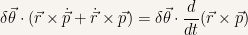 and , it follows
  .
.
Since  is an arbitrary vector it follows
  . Hence
  is constant.
In conclusion one can say that space isotropy implies the conservation of angular momentum. Another important result is that whenever a mechanical system has a symmetry axis the angular momentum about that axis is a conserved quantity.
— 9. Hamiltonian Dynamics —
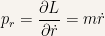
As was seen previously if the potential energy of a system doesn’t depend on velocity then . Consequently one can introduce the following definition:
Definition 8 In a system of generalized coordinates  the generalized momentum is given by the following expression the generalized momentum is given by the following expression
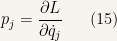
|
As a consequence of the previous definition it is  .
.
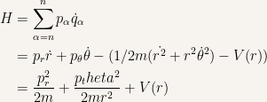
And the Hamiltonian can be written as a Legendre Transformation of the Lagrangian
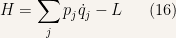
Since  equation 16 can be written

So we have  and
and  . Hence the differential f is
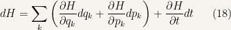
Calculating  and
and  via 16 and substituting into 18 it is

Identifying the coefficients of  ,
,  and
and  it follows:
and

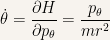
Which are called the canonical equations of motion. When one uses these equations to study the time evolution of a physical system one is using Hamiltonian Dynamics.
One has  . Furthermore one also have
  which implies that if the Hamiltonian function doesn’t depend explicitly on
  then is a conserved quantity.
 and
and  . Then the generalized coordinate is
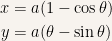
  . Perhaps you might be surprised to find out that we need only a single coordinate to describe the motion of this particle since its motion is described on a plane which is a two dimensional entity. But the particle motion is restricted to be along the ellipse and that constraint decreases the particle’s degrees of freedom to one instead of being two.
  , the distance travelled, and
 and
and  .
. ,
,  ,
,  and
and 
 .
.
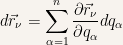
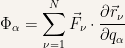
 on its generalized coordinates. Derive the following expression
 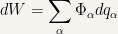 for the total work done by the force and indicate the physical meaning of
  .
.
 it is
it is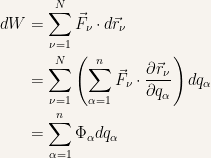
 being the generalized force.
  .
.
 and
and  . Hence
 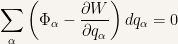 . Since
  are linearly independent it is
  and
and  .
. .
. .
. .
. and
and  .
.
 are connected with each other and to two points
  and
and  by springs with constant factor
  . The particles are free to slide along the direction of
  .
. .
. .
.


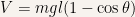
 . The potential is
  .
. 


 to the previous equations

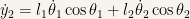
![\displaystyle K=1/2m_1l^2_1\theta^2_1+1/2m\left[ l^2_1\dot{\theta}^2_1+l^2_2\dot{\theta}^2_2+2l_1l_2\dot{\theta}_1\dot{\theta}_2\cos(\theta_1-\theta_2) \right]](https://s0.wp.com/latex.php?latex=%5Cdisplaystyle+K%3D1%2F2m_1l%5E2_1%5Ctheta%5E2_1%2B1%2F2m%5Cleft%5B+l%5E2_1%5Cdot%7B%5Ctheta%7D%5E2_1%2Bl%5E2_2%5Cdot%7B%5Ctheta%7D%5E2_2%2B2l_1l_2%5Cdot%7B%5Ctheta%7D_1%5Cdot%7B%5Ctheta%7D_2%5Ccos%28%5Ctheta_1-%5Ctheta_2%29+%5Cright%5D&bg=f7f3ee&fg=000000&s=0&c=20201002)
![\displaystyle V=m_1g(l_1+l_2-l_1\cos\theta_1)+m_2g\left[l_1+l_2-(l_1\cos\theta_1+l_2\cos\theta_2)\right]](https://s0.wp.com/latex.php?latex=%5Cdisplaystyle++V%3Dm_1g%28l_1%2Bl_2-l_1%5Ccos%5Ctheta_1%29%2Bm_2g%5Cleft%5Bl_1%2Bl_2-%28l_1%5Ccos%5Ctheta_1%2Bl_2%5Ccos%5Ctheta_2%29%5Cright%5D+&bg=f7f3ee&fg=000000&s=0&c=20201002)


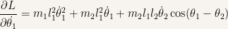
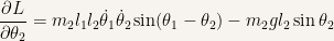
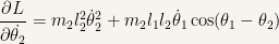


 e
e  and write the equations of motion.
 implies
  and
and  .
.

 subject to a central force that is a function of the distance between the particle and the origin.
 and
and  .
. .
.


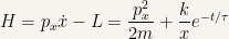
 are positive constants. Find the lagrangian and the hamiltonian.
 it follows
  .
. . Hence the lagrangian is
 .
. .
. it is
it is  .
. and
and  . The Poisson brackets are defined as:
![\displaystyle [g,h]=\sum_k \left(\frac{\partial g}{\partial q_k}\frac{\partial h}{\partial p_k}-\frac{\partial g}{\partial p_k}\frac{\partial h}{\partial q_k}\right)](https://s0.wp.com/latex.php?latex=%5Cdisplaystyle+%5Bg%2Ch%5D%3D%5Csum_k+%5Cleft%28%5Cfrac%7B%5Cpartial+g%7D%7B%5Cpartial+q_k%7D%5Cfrac%7B%5Cpartial+h%7D%7B%5Cpartial+p_k%7D-%5Cfrac%7B%5Cpartial+g%7D%7B%5Cpartial+p_k%7D%5Cfrac%7B%5Cpartial+h%7D%7B%5Cpartial+q_k%7D%5Cright%29+&bg=f7f3ee&fg=000000&s=0&c=20201002)
![{\dfrac{dg}{dt}=[g,H]+\dfrac{\partial g}{\partial t}}](https://s0.wp.com/latex.php?latex=%7B%5Cdfrac%7Bdg%7D%7Bdt%7D%3D%5Bg%2CH%5D%2B%5Cdfrac%7B%5Cpartial+g%7D%7B%5Cpartial+t%7D%7D&bg=f7f3ee&fg=000000&s=0&c=20201002) .
.
![{\dot{q}_j=[q_j,H]}](https://s0.wp.com/latex.php?latex=%7B%5Cdot%7Bq%7D_j%3D%5Bq_j%2CH%5D%7D&bg=f7f3ee&fg=000000&s=0&c=20201002) e
e ![{\dot{p}_j=[p_j,H]}](https://s0.wp.com/latex.php?latex=%7B%5Cdot%7Bp%7D_j%3D%5Bp_j%2CH%5D%7D&bg=f7f3ee&fg=000000&s=0&c=20201002) .
.
![{[p_k,p_j]=0}](https://s0.wp.com/latex.php?latex=%7B%5Bp_k%2Cp_j%5D%3D0%7D&bg=f7f3ee&fg=000000&s=0&c=20201002) e
e ![{[q_k,q_j]=0}](https://s0.wp.com/latex.php?latex=%7B%5Bq_k%2Cq_j%5D%3D0%7D&bg=f7f3ee&fg=000000&s=0&c=20201002) .
.
![{[q_k,p_j]=\delta_{ij}}](https://s0.wp.com/latex.php?latex=%7B%5Bq_k%2Cp_j%5D%3D%5Cdelta_%7Bij%7D%7D&bg=f7f3ee&fg=000000&s=0&c=20201002) .
.
 doesn’t depend explicitly on time and
 ![{[f,H]=0}](https://s0.wp.com/latex.php?latex=%7B%5Bf%2CH%5D%3D0%7D&bg=f7f3ee&fg=000000&s=0&c=20201002) the function is a constant of movement.
the function is a constant of movement.
 with
with  positive constants and
  . Show that:
 and
and  it is
it is

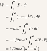
 . Suppose that for
  e
e  the velocities are
  and
and  , respectively. Show that the work the force does on the particle equals its change in kinetic energy.

 .
. . Let
. Let  and
and 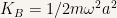
 . Do you see why?
 and
and  is its instantaneous velocity then the instantaneous power is

 . Hence
 is independent of a particle’s trajectory if and only if
  .
.
 denote a closed curve and admit that
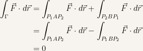
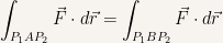 .
.  . If the particle’s positions are
  and
and  on
on  is the total energy then
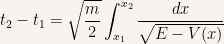
 solve in order to
  from an height
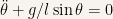
  . Derive the particle’s equation of motion
  .
.
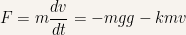 with
with  and
and  . Then solve in order to
  and integrate to find
 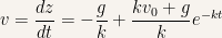 (the terminal velocity
  is
is 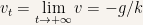 ).
). and integrating and it is
  .
. 
 it follows that
 . Since
  is a constant in our example
 . The generalized coordinates are
  and the generalized momenta are
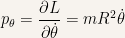

 ,
,  . But
. But 


 . Which is equivalent to saying that the
  with
with  . Which means that the particle describes an harmonic motion along the
  and
and  are called cyclical coordinates.
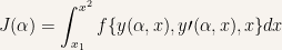
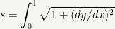
 . Suppose that
  is a functional and the goal of the Calculus of Variations is to determine
  such that the value of
  be a parametric representation of
  such that
  is the function that makes
  , where
  is a function of
  (that means that
  is a continuous function whose derivative is also continuous) with
 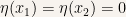 .
.
 . Take
 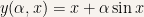 as a parametric representation of
  ,
,  and
and  .
.
 such that
  and
and 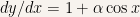 .
.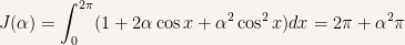 .
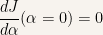
. it is trivial to see that the minimum value is reached when
 and
and  , calculate the equation of the curve that minimizes the distance between the points
 .
. ,
, 
 with
with  .
.
 and
and  it follows
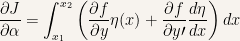
 .
. since
since 
 and taking into account the fact that
 and goes to point
  .
.
 . Let us take our original point as being our reference point for the potential. Then it is
  .
. . For the potential it is
  . From the previous equations it follows that
  .
.
 since
since  is only a constant factor and can be omitted from our analysis. Given the functional form of
  and Euler’s Equation just is:

 it follows
  . Hence the expression for
  . Since our particle starts from the origin it is
  .
.
 variables —
  .
. and
and 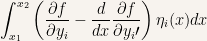 for each of the values of
  . Since
  are independent functions it follows that for
 , of a particle’s movement (be it a real or virtual one) is:
 the actual path that the particle takes is the one that makes the action stationary
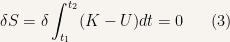
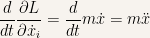
 ,
,  , so
, so  (where
  is called Newton’s notation).


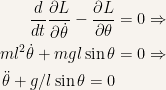
 .
. .
.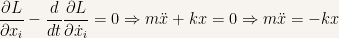 which is just the harmonic oscillator dynamic equation that we already know.
 quantities to describe the position of all particles (since we have 3 degrees of freedom). In the case of having any kind of restraints on the motion of the particles the number of quantities needed to describe the motion of particle is less than
  .
. . These
  coordinates don’t need to be rectangular, polar, cylindrical nor spherical. These coordinates can be of any kind provided that they completely specify the mechanical state of the system.

 ,
,  the number generalized coordinates
  .
.
 equations of constraint
 .
. whose center is the origin of the coordinate system.
 and
and  .
. ,
,  and
and  be our generalized coordinates.
 as a constraint equation. Hence

 .
.


 and
and 
 . Thus the lagrangian is
 it is
it is  . Hence it is
 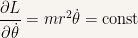 .
. . Thus
  expresses the conservation of angular momentum about the axis of symmetry of system.
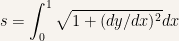 with
with 
 be a constant vector such as
  . Then
  . Hence
  is constant.
 since
since  is parallel to
  and the vector product of two parallel vectors is
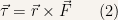

 by definition.
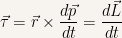 .
. ,
,  and
and  is constant in time.
 to mechanical state
  .
.

 is a total differential (note that we assumed that
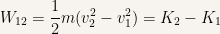


 it is
it is
 and the mechanical system is said to be conservative.
 , created by a body of mass
  in all points of space (except on the point where the particle is situated) which is responsible for the gravitational interaction.
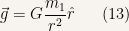
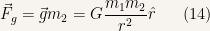
 interacts with a gravitic field
  :
:
 is a unit vector whose direction points from the position of
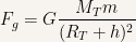
 holds for body of constant mass, one can write for the intensity of gravitational acceleration:
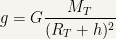

 .
. .
.

 one can write:
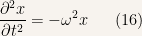
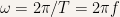
 where
where  e
e  .
.

 is the minimum distance between two points in a wave that are in the same mechanical state.

 :
:
 and
and  are solutions of equation
  , while a wave that moves to the left is always of the form
  .
.

 .
.


 the phenomenom that occurs is called diffraction. Each portion of the slit acts as if it is an independent source of a propagation and as a consequence waves coming from different portions of the slit have different phases. From this interaction one can observe destructive or constructive interference.
 and in general it is proportional to
  where
where  represents an infinitesimal displacement.
 . In classical mechanics the mass of a body its a measure of its resistance to alter its state of movement. This characteristic has the name of inertia.
![{\left[ L \right] =m}](https://s0.wp.com/latex.php?latex=%7B%5Cleft%5B+L+%5Cright%5D+%3Dm%7D&bg=f7f3ee&fg=000000&s=0&c=20201002)
![{\left[ T \right] =s}](https://s0.wp.com/latex.php?latex=%7B%5Cleft%5B+T+%5Cright%5D+%3Ds%7D&bg=f7f3ee&fg=000000&s=0&c=20201002)
![{\left[ M \right] = \mathrm{Kg}}](https://s0.wp.com/latex.php?latex=%7B%5Cleft%5B+M+%5Cright%5D+%3D+%5Cmathrm%7BKg%7D%7D&bg=f7f3ee&fg=000000&s=0&c=20201002)
 .
.


 .
. (force that object
  but opposite direction


 is also an unknown function the calculation has to stop.
 is constant in time (uniformly accelerated motion) we can solve equation
  . After substituting in equation
 the motion is said to be uniform.
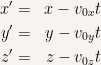
 be two inertial frames whose origins coincide at
  . Moreover
  relative to
 which we can write in component form: